A WorldDynamics tutorial

WorldDynamics allows the user to play with the World3 model introduced in the book Dynamics of Growth in a Finite World (1974). Informally speaking, this model is formed by five systems, each containing one or more subsystems. The following picture shows the structure of the model and the connections between the subsystems which share a common variable.

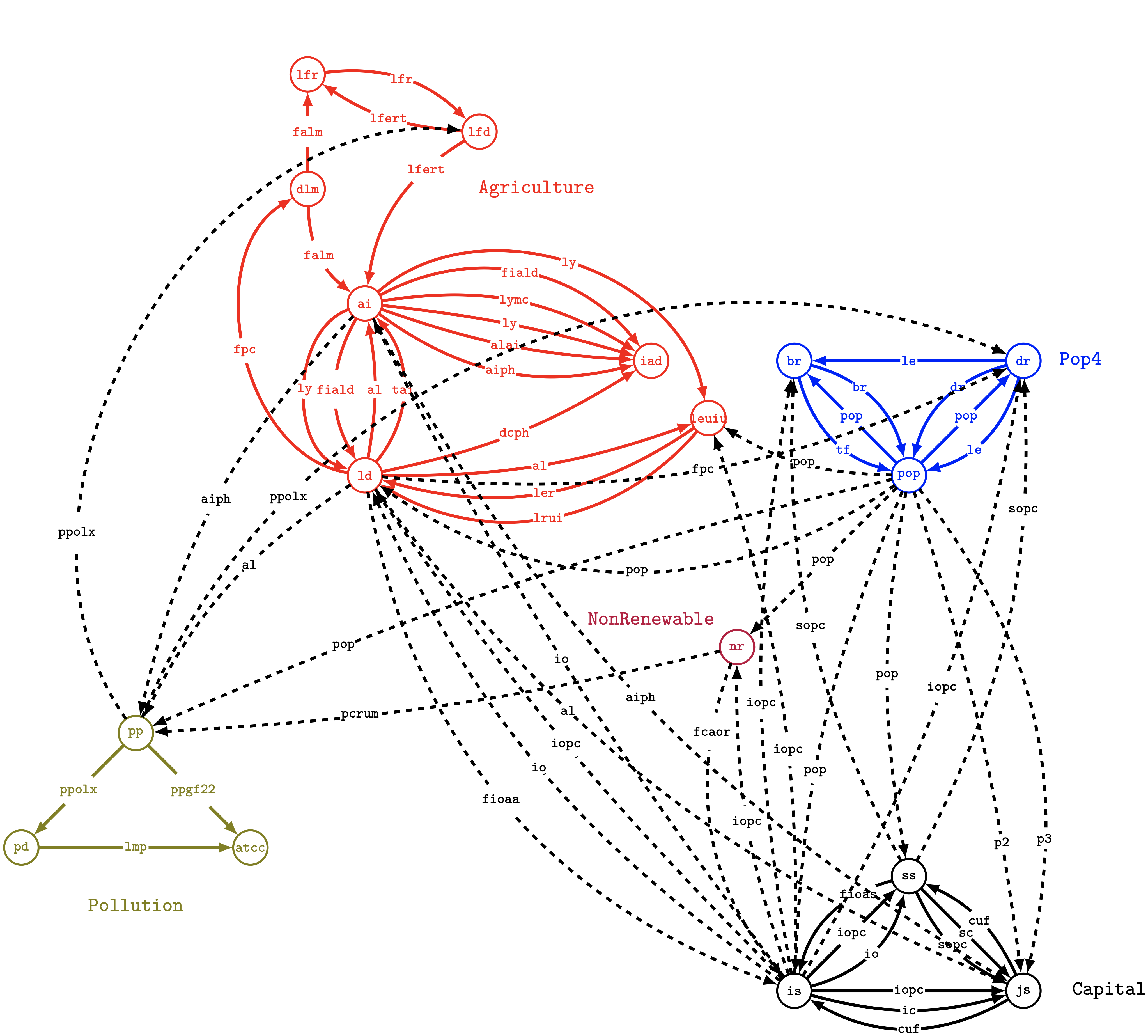
As it can be seen, the five systems are Pop4 (which is the population system with four age levels), Agriculture, Capital, Non-renewable (resources), and Pollution. The Pop4 system is formed by the three subsystems pop (population), br (birth rate), and dr (death rate). For instance, the subsystem br uses the variable pop which originates from the subsystem pop, while the subsystem pop uses the variable le which originates from the subsystem dr. Of course, there are variables which connect subsystem of different systems. For example, the subsystem pp of the system Pollution uses the variable aiph which originates from the subsystem ai of the system Agriculture (for an entire list of variables and of subsystems using them see the World 3 equations, variables, and parameters page).

In WorldDynamics each system is a Julia module and each subsystem corresponds to a Julia function of this module (or of a module which is included in this module), which defines the ODE system corresponding to the subsystem itself. All the ODE systems corresponding to the subsystems of the World3 model have to be composed (see the function compose in the solvesystems.jl code file). This will produce the entire ODE system of the World3 model, which can then be solved by using the function solve in the solvesystems.jl code file.

Let us now see how we can replicate the runs described in the chapters of the above mentioned book.

Replicating book runs

For each run described in the seventh chapter of the book, WorldDynamics defines a function which allows the user to reproduce the corresponding figure. For example, in order to replicate Run 7-1, which shows the behavior of important variables in the population system when the world model is run from 1900 to 1970, and which is described in Section 7.2 of the book and depicted in Figure 7-2, we can simply execute the following code.

using WorldDynamics
World3.fig_2()

Instead, in order to replicate Run 7-28, which reaches equilibrium through discrete policy changes, and which is described in Section 7.7 of the book depicted in Figure 7-38, we can execute the following code.

using WorldDynamics
World3.fig_38()

We can also replicate the runs of the other chapters of the book (each one devoted to one system of the model). For example, in order to replicate the standard run of the capital system, which is described in Section 3.7 of the book and depicted in Figure 3-36, we can execute the following code.

using WorldDynamics
World3.Capital.fig_36()

Performing sensitivity tests

In order to perform sensitivity tests, we have first to modify the parameter or the interpolation table of the variable with respect to which we want to perform the sensitivity test, then to create the ODE system corresponding to the historical run with the modification integrated in the system, and finally to solve the ODE system. We can then plot the resulting evolution of the model.

Modifying a parameter of the variable

In order to reproduce Figure 7-10, for example, in which the nonrenewable resources initial value (that is, the value of the NRI parameter) is doubled, we can modify the value of this parameter by getting the parameter set of the nonrenewable resources sector, and by changing the value of NRI, as shown in the following code.

using WorldDynamics

nonrenewable_parameters_7_10 = World3.NonRenewable.getparameters();
nonrenewable_parameters_7_10[:nri] = 2.0 * nonrenewable_parameters_7_10[:nri];

Creating the ODE system

The ODE system is then created by executing the following code, in which we specify which set of parameter values has to be used for the nonrenewable resources sector.

system = World3.historicalrun(nonrenewable_params=nonrenewable_parameters_7_10);

Solving the ODE system

We then have to solve the ODE system, by executing the following code.

sol = WorldDynamics.solve(system, (1900, 2100));

Plotting the evolution of the model

We first have to define the variables that we want to plot. For example, Figure 7-10 of the book shows the plot of seven variables of seven different subsystems of the model. In order to easily access to these variables, we first create shortcuts to the subsystems in which they are introduced.

using ModelingToolkit

@named pop = World3.Pop4.population();
@named br = World3.Pop4.birth_rate();
@named dr = World3.Pop4.death_rate();
@named is = World3.Capital.industrial_subsector();
@named ld = World3.Agriculture.land_development();
@named nr = World3.NonRenewable.non_renewable();
@named pp = World3.Pollution.persistent_pollution();

The seven variables are then defined as follows.

reference_variables = [
    (nr.nrfr, 0, 1, "nrfr"),
    (is.iopc, 0, 1000, "iopc"),
    (ld.fpc, 0, 1000, "fpc"),
    (pop.pop, 0, 16e9, "pop"),
    (pp.ppolx, 0, 32, "ppolx"),
    (br.cbr, 0, 50, "cbr"),
    (dr.cdr, 0, 50, "cdr"),
];
@variables t;

For each variable that we want to plot, the above vector includes a quadruple, containing the Julia variable, its range, and its symbolic name to be shown in the plot (the range and the symbolic name are optional). The time variable t has also to be declared.

Finally, we can plot the evolution of the variables according to the previously computed solution.

plotvariables(sol, (t, 1900, 2100), reference_variables, title="Fig. 7-10", showlegend=true, colored=true)

Modifying an interpolation table

In order to reproduce Figure 7-13, in which the slope of the fraction of industrial output allocated to agriculture is increased, we can modify the two tables FIOAA1 and FIOAA2 by getting the table set of the agriculture sector, and by changing the value of these two tables. We then have to solve the ODE system again, by specifying which set of tables has to be used for the agriculture sector. Finally, we can plot the same seven variables of Figure 7-10. This is exactly what we do in the following code.

using WorldDynamics

agriculture_tables_7_13 = World3.Agriculture.gettables();
agriculture_tables_7_13[:fioaa1] = (0.5, 0.3, 0.1, 0.0, 0.0, 0.0);
agriculture_tables_7_13[:fioaa2] = (0.5, 0.3, 0.1, 0.0, 0.0, 0.0);
system = World3.historicalrun(agriculture_tables=agriculture_tables_7_13);
sol = WorldDynamics.solve(system, (1900, 2100));
plotvariables(sol, (t, 1900, 2100), reference_variables, title="Fig. 7-13", showlegend=true, colored=true)

Updating the model with modern data

The flexible structure of WorldDynamics allows the user to feed the model with modern data. For example, in the book, the variable POP of the pollution system is assigned the following interpolation table which corresponds to the population number (expressed in $10^8$) for a set of years between 1900 and 2100.

tables[:pop] = (16.0, 19.0, 22.0, 31.0, 42.0, 53.0, 67.0, 86.0, 109.0, 139.0, 176.0);
ranges[:pop] = (1900, 2100)

Instead, we can extend the above set of years to a much larger one as well as replace any outdated estimations with more recent data available at open-source data catalogs. In the following, we consider past and future projections of the world population, taken from the recognized public database Our World In Data. We first have to modify the table POP by getting the table set of the pollution sector, and by changing its value. We then have to solve the ODE system again, by specifying which set of tables has to be used for the pollution sector. This is exactly what we do in the following code.

using WorldDynamics

tables = Pollution.gettables();
tables[:pop] = (16.47,16.59,16.73,16.87,17.02,17.16,17.31,17.47,17.62,17.77,17.93,18.05,18.18,18.30,18.43,18.56,18.69,18.82,18.95,19.09,19.26,19.40,19.56,19.73,19.90,20.08,20.26,20.44,20.63,20.82,21.04,21.22,21.44,21.66,21.88,22.10,22.33,22.57,22.80,23.03,23.27,23.45,23.64,23.82,24.00,24.17,24.35,24.54,24.75,25.01,24.99,25.43,25.90,26.40,26.92,27.46,28.01,28.58,29.16,29.70,30.19,30.68,31.27,31.96,32.67,33.37,34.06,34.75,35.47,36.21,36.95,37.70,38.45,39.20,39.96,40.69,41.43,42.16,42.90,43.66,44.44,45.25,46.08,46.92,47.76,48.62,49.50,50.41,51.32,52.24,53.16,54.06,54.93,55.77,56.61,57.43,58.25,59.06,59.87,60.68,61.49,62.31,63.12,63.94,64.76,65.58,66.41,67.26,68.12,68.98,69.86,70.73,71.62,72.51,73.39,74.27,75.13,76.00,76.84,77.65,78.41,79.09,79.75,80.45,81.19,81.92,82.64,83.36,84.07,84.77,85.46,86.15,86.82,87.49,88.15,88.79,89.43,90.06,90.68,91.29,91.88,92.47,93.04,93.60,94.14,94.68,95.19,95.69,96.18,96.65,97.09,97.53,97.94,98.34,98.72,99.08,99.43,99.76,100.08,100.39,100.68,100.96,101.22,101.48,101.73,101.96,102.18,102.40,102.60,102.79,102.97,103.14,103.30,103.45,103.59,103.71,103.82,103.92,104.01,104.08,104.15,104.20,104.24,104.27,104.29,104.31,104.31,104.30,104.29,104.27,104.24,104.20,104.15,104.09,104.03,103.96,103.89,103.80,103.70,103.60,103.49);

system = World3.Pollution.historicalrun(tables=tables);
sol = WorldDynamics.solve(system, (1900, 2100))

Finally, we can compare the model updated with new data against the one with outdated data by reproducing the figures from the book (as described within the Replicating book runs section).

Implementing a new model

In this final section of the tutorial, we show how we can implement a new model using the WorldDynamics framework. To this aim we refer to the third chapter of the book System Dynamics Modeling with R (2016), by Jim Duggan. In this chapter, whose title is Modeling Limits to Growth, the author introduces the reader to system dynamics models of limits to growth through three models of increasing complexity. Here, we will implement the third model, in which a growing stock consumes its carrying capacity (this dynamic leads to growth followed by rapid decline). In this case we have only one system, called NonRenewableStock, which contains only one subsystem (that is, one ODE system). The coding of this system consists of four Julia source files, that is, subsystems.jl, initialisations.jl, parameters.jl, and tables.jl (we assume that these files will be included in the directory nonrenewablestock contained in the directory Duggan). The first source file will contain the variable and parameter declarations, and the function specifying the ODE system corresponding to the subsystem. The second and third source files will contain the initial values of the variables and the values of the parameters, respectively. Finally, the fourth source file will contain the tables and the ranges used to interpolate a non-linear function through a collection of linear segments.

Coding the parameters

The model uses five parameters whose values are specified in a dictionary declared in the file parameters.jl as follows.

_params = Dict{Symbol,Float64}(
    :cost_per_investment => 2,
    :depreciation_rate => 0.05,
    :fraction_profits_reinvested => 0.12,
    :revenue_per_unit_extracted => 3,
    :desired_growth_fraction => 0.07,
)
getparameters() = copy(_params)

Note that the function getparameters is exactly the one that has been used above while modifying a parameter.

Coding the initial values of the variables

The model uses 12 variables: two of them requires to specify their initial values. This is done in a dictionary declared in the file initialisations.jl as follows.

_inits = Dict{Symbol,Float64}(
    :capital => 5,
    :resource => 1000,
)
getinitialisations() = copy(_inits)

Note that the function getinitialisations can be used to get a copy of the dictionary in order to change some initial values.

Coding the subsystem

The file subsystems.jl starts with the decalaration of the variable t with respect to which the derivatives have to be computed.

@variables t
D = Differential(t)

The file subsystems.jl continues by declaring one function (corresponding to one subsystem, that is, one ODE system) in which all variables and parameters of the subsystem are declared and the ODE system is defined.

function non_renewable_stock(; name, params=_params, inits=_inits, tables=_tables, ranges=_ranges)
    @parameters cost_per_investment = params[:cost_per_investment]
    @parameters depreciation_rate = params[:depreciation_rate]
    @parameters fraction_profits_reinvested = params[:fraction_profits_reinvested]
    @parameters revenue_per_unit_extracted = params[:revenue_per_unit_extracted]
    @parameters desired_growth_fraction = params[:desired_growth_fraction]
    @variables capital(t) = inits[:capital]
    @variables depreciation(t)
    @variables desired_investment(t)
    @variables resource(t) = inits[:resource]
    @variables extraction(t)
    @variables extraction_efficiency_per_unit_capital(t)
    @variables total_revenue(t)
    @variables capital_costs(t)
    @variables profit(t)
    @variables capital_funds(t)
    @variables maximum_investment(t)
    @variables investment(t)
    eqs = [
        D(capital) ~ investment - depreciation
        depreciation ~ capital * depreciation_rate
        desired_investment ~ desired_growth_fraction * capital
        D(resource) ~ -extraction
        extraction ~ capital * extraction_efficiency_per_unit_capital
        extraction_efficiency_per_unit_capital ~ interpolate(resource, tables[:eepuc], ranges[:eepuc])
        total_revenue ~ revenue_per_unit_extracted * extraction
        capital_costs ~ capital * 0.10
        profit ~ total_revenue - capital_costs
        capital_funds ~ profit * fraction_profits_reinvested
        maximum_investment ~ capital_funds / cost_per_investment
        investment ~ min(desired_investment, maximum_investment)
    ]
    ODESystem(eqs, t; name)
end

The arguments of the function are the dictionaries corresponding to the variable initial values and to the parameter values, and the dictionaries corresponding to the tables and the ranges used for the linear of non-linear functions. The first two dictionaries are used to assign a value to all the parameters and an initial value to two variables. The ODE system is a vector of differential and algebraic equations (as specified in the chapter of the above mentioned book). Note that the two differential equations correspond to the two variables whose initial value has been specified. The variable extraction_efficiency_per_unit_capital is defined as a linear interpolation of the variable resource, by using the table tables[:eepuc] together with the range ranges[:eepuc]. The table and the corresponding range are defined in the file tables.jl, which define two dictionaries as follows.

_tables = Dict{Symbol,Tuple{Vararg{Float64}}}(
    :eepuc => (0.0, 0.25, 0.45, 0.63, 0.75, 0.85, 0.92, 0.96, 0.98, 0.99, 1.0),
)
_ranges = Dict{Symbol,Tuple{Float64,Float64}}(
    :eepuc => (0.0, 1000.0),
)
gettables() = copy(_tables)
getranges() = copy(_ranges)

Note that the function gettables is exactly the one that has been used above while updating a model with modern data.

We can now define a scenario by simply invoking the function non_renewable_stock and by returning the ODE system returned by this function. This is done in the file scenarios.jl (we assume that also this file is contained in the directory nonrenewablestock) which contains the following code.

function nrs_run(; kwargs...)
    @named nrs = non_renewable_stock(; kwargs...)
    return nrs
end

Observe that if the model contains multiple systems and/or multiple subsystems, then the ODE systems returned by all the subsystems have to be composed by using the function compose (which also asks for the connections between the variables declared and used in different subsystems). An example of a scenario using multiple systems and subsystems is defined in the file scenarios.jl included in the directory world2 within the World model directory.

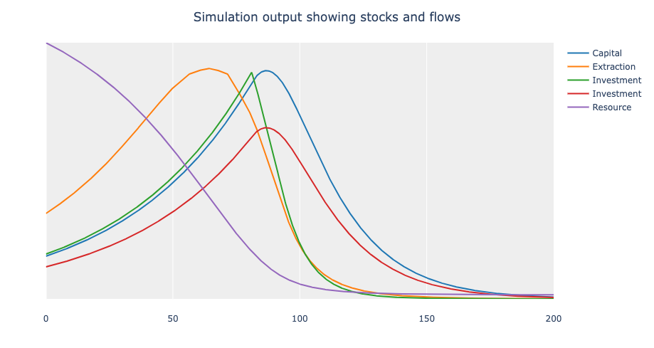
Finally, the model can be solved and simulated by using the solve and the plotvariables functions that we already used above. In particular, the file plots.jl (we assume that also this file is contained in the directory nonrenewablestock) does it in order to reproduce Figure 3.9 of the chapter of the above mentioned book.

using ModelingToolkit
using DifferentialEquations

function nrs_run_solution()
    isdefined(@__MODULE__, :_solution_nrs_run) && return _solution_nrs_run
    global _solution_nrs_run = WorldDynamics.solve(nrs_run(), (0, 200), solver=Tsit5(), dt=0.015625, dtmax=0.015625)
    return _solution_nrs_run
end
function _variables_nrs()
    @named nrs = non_renewable_stock()
    variables = [
        (nrs.capital, 0, 30, "Capital"),
        (nrs.extraction, 0, 15, "Extraction"),
        (nrs.investment, 0, 2, "Investment"),
        (nrs.depreciation, 0, 2, "Investment"),
        (nrs.resource, 0, 1000, "Resource"),
    ]
    return variables
end

fig_3_9(; kwargs...) = plotvariables(nrs_run_solution(), (t, 0, 200), _variables_nrs(); title="Simulation output showing stocks and flows", showaxis=false, showlegend=true, kwargs...)

Note that, for performance reasons, the definition of the function nrs_run_solution starts by checking whether the solution of the model is already available: in this case, nothing is done.

Creating the new model module

We can now define a Julia module Duggan.jl as follows (we assume that this source file is contained in the directory Duggan).

module Duggan
using ModelingToolkit
using WorldDynamics
include("NonRenewableStock.jl")
end

The file NonRenewableStock.jl (we assume that also this file is contained in the directory Duggan) simply includes all the Julia source files we have written above.

module NonRenewableStock
using WorldDynamics
using ModelingToolkit
include("nonrenewablestock/tables.jl")
include("nonrenewablestock/parameters.jl")
include("nonrenewablestock/initialisations.jl")
include("nonrenewablestock/subsystems.jl")
include("nonrenewablestock/scenarios.jl")
include("nonrenewablestock/plots.jl")
end

Solving the model and producing the figure

We assume that we execute the Julia REPL from the directory containing the folder Duggan. We can solve the model and produce the desired figure by simply executing the following two instructions.

using WorldDynamics
Duggan.NonRenewableStock.fig_3_9()

If everything worked well, the following picture should be shown.